Perhaps one of the most puzzling phenomena to see for the first time in quantum mechanics is that of a
particle tunneling through a barrier. Classically, there is no explanation for how a particle such as an electron
could penetrate a barrier. Only by considering the electron as both a particle and a wave can one obtain a
physical model that explains electron tunneling.
Many examples of electron tunneling can be found in everyday life. As mentioned in class, a large part of
the heat generated by your laptop is from electrons tunneling through the gates of transistors in modern
microprocessors. Figure 1 shows a cross-section of a modern transistor. The single-ended arrow points to
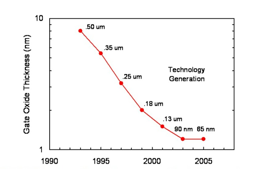
the gate oxide of only a few nanometers in thickness. Figure 2 shows the scaling of the gate oxide thickness
over the last several generations of MOSFETs.
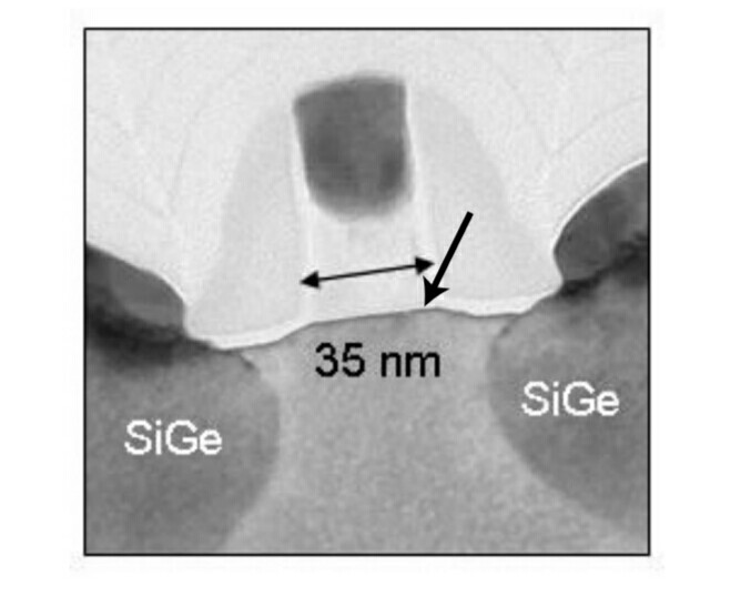
ters. The single-ended arrow points to the thin gate oxide layer.
The nominal channel length for each generation is indicated.
An additional everyday example of electron tunneling occurs in flash-based storage, such as in the memory
cards for digital cameras and in flash-memory-based MP3 players. Figure 3 shows a schematic of a flash
memory device. In flash memory, the discharging of electrons on the floating gate occurs through a tunneling
process.
Describing Tunneling Current – Fowler-Nordheim Equation
As you’ll learn in 6.002 and 6.012, one of the primary means for characterizing electrical devices is to
determine the amount of current that flows through the device for a given applied voltage. The plots of
current (I) versus voltage (V) that you can generate for various devices are known as I-V characteristics. For
electron tunneling, also referred to in scientific literature as “field emission,” the I-V characteristic can be
derived using a the simple barrier tunneling picture that we went over in class. By making some simplifying
assumptions, an I-V relationship known as the Fowler-Nordheim Formula can be derived.
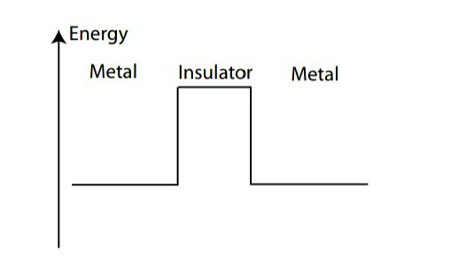
Consider the system shown in Figure 4. Two regions of metal are separated by an insulting material. The
potential energy of each section and how they relate to one another are shown by the sketched levels. Without
an applied field (or voltage), the energies of all the levels are flat.
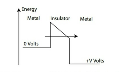
However, when a low field is applied, the metal energy levels shift with respect to one another in energy
by the applied potential as shown in Figure 5. Recall that ∆U = q∆V , and since we are talking about
electrons, q = −e, so a material at a higher voltage has electrons with lower potential energy. This difference
in energy is dropped linearly over the insulator (corresponding to a constant electric field in the insulator
region).
Finally, when a very high electric field is applied, the barrier becomes triangular since the difference in
potential energies between the two metals is very high as shown in figure. This is the system used to
derive the Fowler-Nordheim Formula.
making the barrier between the metals resemble a trapezoid.
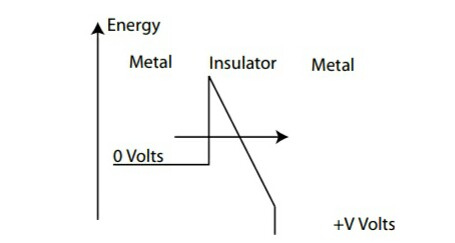
between the metal regions is triangular.
We won’t delve into the derivation of the Fowler-Nordheim Formula here since it relies on a more advanced
quantum mechanics tool known as the WKB approximation to model the triangular potential barrier. The
WKB approximation is covered in classes like 6.728.
By computing the probability current through an approximation of the barrier as a triangle (making use of
the WKB approximation), the formula for current versus voltage is found to be of the form:
I = AK1V
2
e
−K2/V
where I is the current, A is the cross-sectional area of the material, V is the applied voltage between the
metal regions, and K1 and K2 are constants that depend on the underlying material properties and the
length of the insulator region.
The above is the Fowler-Nordheim Formula. As you can see from the formula above, when tunneling is the
dominant conduction mechanism, the I-V characteristic is no longer that of Ohm’s law, the linear relation
V = IR. Instead, the resistance effectively changes as a function of applied voltage. We can define the
resistance in this case as
∂V R(Vi) = ∂I |Vi
